This is a part of the series of blogs on the basics of molecular modelling. The QM program GAMESS is used for the calculations. This post follows part 4, where the optimization of a transition state(TS) is described. In this part, we will perform an intrinsic reaction coordinate (IRC) calculation on that TS.
IRC is basically a method that we can use to confirm if we actually have the transition state that we wanted. The TS from the calculation represents a geometry where the energy w.r.t. one vibrational mode is the maximum, and for all other vibrational modes, the energy is minimum: a saddle point. What IRC does is that it takes the TS, and then slowly moves along the vibrational mode that has the imaginary frequency, while allowing other coordinates to relax. This means that we effectively follow the minimum energy path going down on either side from the TS. The IRC stops when on the energy path becomes flat i.e. the reactant or product state is reached.

IRC follows the minimum energy path from TS

What we get at each end, should be close to the structures of the reactants and products. If the structures at the ends of IRC are not what we expect, it suggests that something is wrong with the TS (most probably the wrong TS was chosen to start with).

For this post, we will use GAMESS and wxMacMolPlt.

Preparing input files for IRC

In GAMESS to run an IRC, we need the structure of the transition state, and the hessian (force constants) for that transition state. Let’s continue from the TS for the Diels-Alder reaction that was obtained in Part 4 of this blog series.

Open the output file with wxMacMolPlt, and use Subwindow>Input builder to write an input file. It doesn’t matter what options you choose, because we will edit the input file after this. You can use Notepad to edit.

To run an IRC we need to set RUNTYP=IRC in $CONTRL, and also put in an $IRC group. The top of the input file that I used:

$CONTRL SCFTYP=RHF RUNTYP=IRC MAXIT=60 NZVAR=1 $END
 $SYSTEM MWORDS=20 PARALL=.TRUE. $END
 $BASIS GBASIS=PM6 $END
 $PCM SMD=.t. SOLVNT=DIOXANE $END
 $ZMAT NONVDW(1)=3,10, 4,12 DLC=.t. AUTO=.t. $END
 $IRC PACE=GS2 OPTTOL=0.0001 MXOPT=300 STRIDE=0.10 NPOINT=300
 TSENGY=.t. SADDLE=.t. FORWRD=.t. NPRT=-2 $END

We are using the same semi-empirical method PM6 that we used for the TS optimization. This is important! You can’t use different methods for optimization and IRC. The same solvent dioxane is included with $PCM, as we did in the optimization. About 20 megawords(=16 MB) of RAM is assigned in $SYSTEM. The maximum number of SCF iterations(MAXIT) is set to 60, just to be safe, usually SCF converges in less than 40 iterations. As we are using redundant internal coordinates, the two bonds that are formed/detached have to be read in by NONVDW (as the distance is too large for the program to automatically detect)

In the $IRC group, PACE=GS2 requests the use of Gonzalez-Schlegel 2nd order algorithm for IRC, this is the most efficient algorithm present in GAMESS, however, it needs the accurate hessian at the TS to work. OPTTOL represents the convergence criteria to determine if the IRC has reached the lowest energy on any side of the TS. MXOPT sets the number of constrained optimizations that GS2 will perform on each IRC point. Setting a large number for this is beneficial. STRIDE is the size of each step that the algorithm takes on the potential energy surface. The default value in GAMESS is 0.30, but it’s good to set it to a lower value, such as 0.10. Smaller steps usually means the constrained optimizations converge quickly. In difficult cases, values as small as 0.05, or 0.01 may help. NPOINT sets the number of IRC points that will be determined. This can be set to any large number, because the algorithm will stop automatically as soon as the lowest energy geometry on one side of the TS is encountered. Finally SADDLE=.t. tells the program that the geometry supplied is the transition state, and FORWRD=.t. tells the IRC to go in the forward direction from the TS. (What forward and reverse means is not really important, and may not have any link to reactant or product side. But setting forward in one run and reverse in other run will give you both sides of the IRC).

You will then need to create a copy of the same input file and make FORWRD=.f. for the reverse IRC.

[For a description of what the keywords mean, always refer to the GAMESS documentation that you can find inside the GAMESS folder. There is also an out-of-date online version here. You can also use the previous parts of this blog series, I always provide short descriptions of all the keywords used.]

Hessian of the TS

The GS2 algorithm needs the hessian calculated at the TS for the IRC to run. This hessian has to be put in by $HESS group in the input file.

To get the hessian, you need to look in the restart subfolder in the GAMESS folder. There should be a .dat file with the same name as your input file for the TS optimization. Open that file with Notepad. Now search for $HESS with the find tool in notepad. There might be more than one, in which case, you have to take the last one. It should look like this:

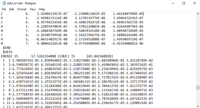
There will be some lines after $HESS, and then the group will end with an $END. You have to copy the whole group. (Be careful that you are not copying text from any other section)
Then paste the $HESS group into both of the input files. We can now run those input files. It should not take more than 10 minutes for the two calculations.

IRC Path

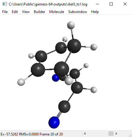
We can now analyze the output files with MacMolPlt. Open the forward IRC file. You can use the slider at the bottom to see all the IRC points that the program has generated:

The end structure does look like the product that we expect for a Diels-Alder reaction, so that’s good!
The energies of the points on the IRC can be seen from Subwindow>Energy plot. This is usually a smooth curve.

You can then open the open the reverse IRC file and look at the structures and energies to make sure that it is going towards the reactants.

Running IRC without hessian

It’s always easier to run the IRC with a $HESS group. But if for some reason, the .dat file is lost, but the TS optimization output file is available, then there is another way to run the IRC. This is not as efficient as running with a $HESS, and also I have not tested it a lot, so I am not sure if there are any accuracy issues. (Most other QM programs like Gaussian only allow an IRC run with hessian.)

To do this, we need the frequency of the imaginary vibration mode, and it’s components in cartesian form. Open the TS output file with notepad, and search for ‘NORMAL COORDINATE ANALYSIS’. Then scroll down until you find the frequencies and their cartesian components:

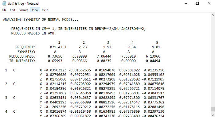
The imaginary frequency will have an ‘I’ next to it. Now you have to copy each of the components X,Y, and Z that are on the same column as the frequency. Then paste them in the input file with the CMODE keyword in $IRC group:

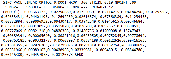
The order of the numbers has to be the same as in the output file from top to bottom, otherwise it will not work. Copying the numbers can be a painstaking work, particularly for large systems. In those cases, it is probably better to automate it with a script. After this, the value of the imaginary frequency also needs to be input with FREQ.
Unfortunately, GS2 algorithm does not work with this, so other algorithms have to be used. I have used AMPC4 and LINEAR algorithms, and found both of them to work well. You can experiment with other algorithms in GAMESS and see which one works better for you.

For some reason MacMolPlt cannot open the .log files from these calculations. So instead you have to open the .trj files from the restart directory with MacMolPlt. It will show you the same IRC path and energies.
In the next part of the blog, we will continue with the same reaction, and calculate the Gibbs free energy of activation, something that can be linked to actual experimental data.

wxMacMolPlt: https://brettbode.github.io/wxmacmolplt/
GAMESS: https://www.msg.chem.iastate.edu/gamess/