This is part of the ongoing series of blogs where I write about the how-to of the molecular modelling. This is mainly focused on the software side of it (GAMESS).
Modelling transition states(TS) is important in studying chemistry. Not only can it give data about the Gibbs free energy of activation (which can be used to calculate rates), it can also help in understanding the possible mechanistic pathways, and how different functional groups may alter the reaction rate.
Getting the TS guess structure
To optimize the TS structure, we need a good guess of the TS structure. This is often very difficult, and it requires a good knowledge of chemistry. The QM programs all operate on a garbage-in-garbage-out manner, so if the guess structure is wrong, even if the program detects a transition state, it would not be the right one. So the whole analysis hinges on getting the correct TS guess structure.
Avogadro has multiple tools to draw the guess structure. A good method is to use the constraints feature from Extensions>Molecular Mechanics.
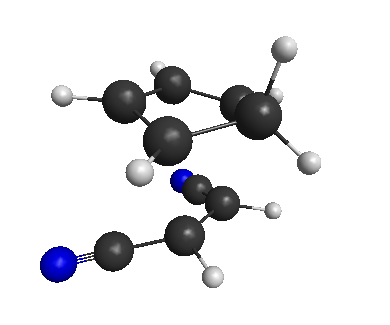
Let’s try to model a transition state for an SN2 like reaction from this paper (The full paper is accessible for free). Let’s proceed with the reaction 33 in Table-3 on page 2677 on the paper. This is a Diels-Alder reaction between cyclopentadiene and maleonitrile (figure below).

The Diels Alder reactions are known to usually go through a transition state where the diene approaches the dienophile from the top, in a concerted mechanism.
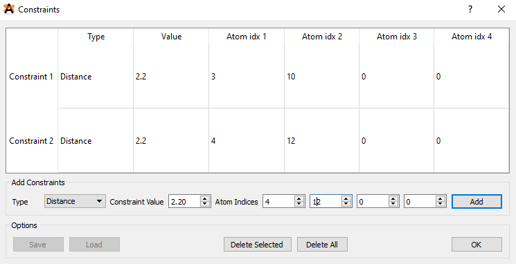
Let’s build the guess structure with Avogadro. In this case, it is easy to start from the product. Draw the product structure. Then use the constraints feature to set the two bonds that will form during the reaction to 2.2Å.
Then optimize the geometry with MMFF94 (or any other force field). You will get something like this:
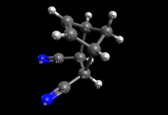
Guess structure for TS optimization
Now how did I come up with the value 2.2Å? Well, there is no way to actually know the value without trying the calculation, but you can guess a value: usually the value is between the sum of the covalent radii and the sum of the van der Waals radii of the atoms that are forming the bond. When in doubt, take the value midway between them. In this case, the bonds are forming between C and C. So, sum of covalent radii=1.4Å, sum of van der Waals radii=3.4Å, average=2.2Å. (There is a way of getting at a better guess structure, by potential energy surface scan. I will write about this in a latter post)
Constrained optimization
Next, what we have to do is to check if the guess structure is close to the transition state. We can do this by constrained optimization. The two bond lengths (which are forming in the TS) are constrained i.e. fixed. Then the rest of the structure is allowed to relax to the lowest energy possible with those constraints in place.
In the paper, geometry optimization is done using B3LYP/6–31G(d). But on your PC, that could take a long time. So, we will use a semi-empirical method — PM6. This method skips some of the computational steps and replaces them with parameters derived from experimental dataset. This makes it very fast, quite accurate, but also prone to massive errors if the dataset did not contain the types of molecules we are dealing with. Fortunately, PM6 is a good general purpose model, parameterized especially for biochemical molecules (In GAMESS, only atoms upto F are supported for PM6).
Prepare the input with Avogadro, and then save it. Then edit the file:
 $CONTRL SCFTYP=RHF RUNTYP=OPTIMIZE MAXIT=60 NZVAR=1 $END
 $SYSTEM MWORDS=80 PARALL=.TRUE. $END
 $BASIS GBASIS=PM6 $END
 $STATPT OPTTOL=0.0004 NSTEP=200 HSSEND=.t. NPRT=-2 $END
 $PCM SMD=.t. SOLVNT=DIOXANE $END
 $FORCE METHOD=SEMINUM $END
 $ZMAT NONVDW(1)=3,7, 4,10 DLC=.t. AUTO=.t.
 IFZMAT(1)=1,3,10, 1,4,12 FVALUE(1)=2.2, 2,2 $END
Here putting GBASIS=PM6 requests a semi-empirical calculation directly. In the paper, the solvent used for this particular reaction is dioxane. We will use the implicit solvation method (fast) SMD to account for the solvent effects. HSSEND=.t. requests the program to calculate the hessian after the optimization is finished.
As the bond distances between 3,7 and 4,10 are too long, we have to explicitly put them in with NONVDW. Then the coordinates to be frozen (constrained) are defined with IFZMAT. Here 1,3,10 means the bond(1) between the atoms numbered 3 and 10. The bonds are both constrained to a value of 2.2Å with FVALUE. (Note that the coordinate system by default works in angstroms for distances and degrees for angles.) As the auto generation of internal coordinates is requested, the value of NZVAR can be set to any value>0, the program automatically determines the number of coordinates required (Part1). The keyword METHOD=SEMINUM is required as PM6 method does not have analytic hessian. So, the hessian has to be calculated by numeric differentiation.
Imaginary frequencies
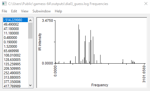
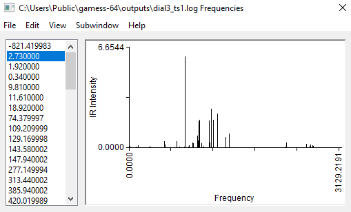
The calculation should not take more than 5 minutes. When it is finished, open the output file with wxMacMolPlt. Go to Subwindow>Frequencies. Then you will see a list of calculated vibrational frequencies. Click on any frequency to see the arrows representing that particular mode of vibration.
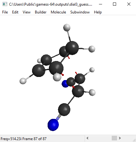
We are looking for the imaginary frequency (represented with a minus sign, but it’s actually imaginary). In this case, this should be the first mode.
You can also see an animation of the vibration from View>Animate Mode. The vibration mode should be such that oscillation in one direction will lead to the product, and oscillation in the other direction leads to the reactants(figure below). Then you have got a good guess for transition state.

Now a bit of theory! The frequencies are basically proportional to the square-root of second derivatives of the energy w.r.t. the displacements along that particular mode. At an energy minimum, the second derivative is positive. But at an energy maximum the second derivative is negative, which means that the frequency is imaginary. The definition of a transition state (or a saddle point) is that there is only one mode of vibration where the energy is maximum, and for all other modes energy is at minimum. If our structure shows only one imaginary frequency, that means the structure is near the TS.
Final TS optimization
With the guess structure, we can start the search for the actual TS. From MacMolPlt you can use Subwindow>Input Builder to write the input file with the coordinates. The options do not matter because we will edit the input file after this.
 $CONTRL SCFTYP=RHF RUNTYP=SADPOINT MAXIT=60 NZVAR=1 $END
 $SYSTEM MWORDS=80 PARALL=.TRUE. $END
 $BASIS GBASIS=PM6 $END
 $STATPT OPTTOL=0.00005 NSTEP=300 HESS=CALC HSSEND=.t.
 IFOLOW=1 NPRT=-2 $END
 $PCM SMD=.t. SOLVNT=DIOXANE $END
 $ZMAT NONVDW(1)=3,7, 4,10 DLC=.t. AUTO=.T. $END
Change runtype to SADPOINT to initate a TS optimization. Add HESS=CALC to request calculation of hessian at the beginning. This is required for a TS search. (In computationally heavy methods, we can read the hessian from the previous calculation, but in this case, it’s not necessary.) In $STATPT, IFOLOW=1 instructs GAMESS to follow the 1st vibrational mode (which is the imaginary one) to the maximum, while allowing other modes to relax. The TS search may converge without this keyword, but it’s useful in cases where other modes also develop imaginary frequencies during the optimization. Change the optimization tolerance to a smaller value, because this is a TS optimization. Finally, remove the constraints from the $ZMAT group, we don’t need them anymore.
Run the TS search, and when it finishes, open it with MacMolPlt and look at the frequencies. Make sure that there is only one imaginary frequency.
The structure should not be too different from the guess structure.
This is the transition state for our reaction!
Multiple imaginary frequencies
If you get more than one imaginary frequencies from the guess structure, then probably the guess structure is probably not close to the actual TS. Its usually recommended that the calculation is restarted with another, better guess structure. Keep in mind though that in many cases frequencies upto -300 can be considered as negligible or zero, as the software can make errors in calculating the frequency.
However, if you are confident that your structure is correct, then you have to look at the vibrational modes, and determine which one leads to the TS. Usually this is the mode with a large imaginary frequency. Then you can have GAMESS follow that mode to its maximum with IFOLOW. Reduce the optimization tolerance to small values to ensure that the other modes are minimized to a sufficient extent. If even after this, your final TS has multiple imaginary frequencies, then you should probably start from the beginning.
In the next post, we will continue from the TS we just got, and perform IRC to determine the reactants and products.
wxMacMolPlt: https://brettbode.github.io/wxmacmolplt/
Avogadro: https://avogadro.cc/
GAMESS: https://www.msg.chem.iastate.edu/gamess/