This is another part of the series of blogs about molecular modelling, mainly about the actual usage of the software, rather than the detailed theory. The QM calculations are done with GAMESS, and visualisation with wxMacMolPlt.
One of the main uses of quantum chemistry is to calculate the Gibbs free energy of activation(ΔG‡) of reactions. This is basically the difference in free energy between the reactant and transition state.
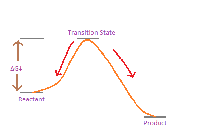
Gibbs free energy of activation for a single step reaction
This is important because we can measure the reaction rates in a lab, and then we can relate the rate to the free energy of activation by a simple mathematical relation: the Eyring-Polanyi equation.
Eyring-Polanyi equation
k_{r}=\frac{\kappa k_{b} T}{h} e^{-\frac{\Delta G^{\dagger}}{R T}}
kᵣ is the rate constant of the reaction, that can be directly measured from experiments. ΔG‡ is the activation energy that can be calculated with the QM software. T is the temperature and the other terms are constants. (Note that for multi-step reactions, it’s a bit more complicated)
This equation provides a powerful link to connect our QM calculations with real-world experimental observations. What is usually done in research is that the ΔG‡ from the experimental kᵣ is compared against the ΔG‡ from QM. If they are close, then it’s likely that the transition state and mechanism that we calculated are a good approximation for what’s happening inside the conical flask. It’s also possible to use QM to predict the rates of reactions that have not been done/cannot be done experimentally.
Modelling the reaction
Before we can calculate the free energy of activation, we must model the whole reaction path. At the very least, there are 4 steps that have to be done:
- Transition state(TS) optimization
- Intrinsic Reaction Coordinate(IRC) calculation, both forward and reverse
- Reactant and product optimization
- Thermochemistry calculation on TS, reactant and product
This is for a reaction that only goes through a single elementary step, without any intermediates. If there are intermediates, then each of the steps in the middle have to be modelled as well. Also, the relation between the rate constant and the QM calculations becomes less straightforward, as there are multiple ΔG‡ for multiple steps.
For now, let’s focus on simple one step reactions. We will continue using the same Diels-Alder reaction from Part 4 and 5 of this blog series:
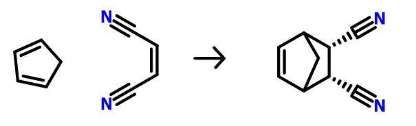
Diels-Alder reaction between cyclopentadiene and maleonitrile
TS optimization
First we have to optimize the transition state (or, what we think is the transition state). I covered how to do this in Part 4. Let’s use the transition state that we obtained with PM6/SMD(dioxane):
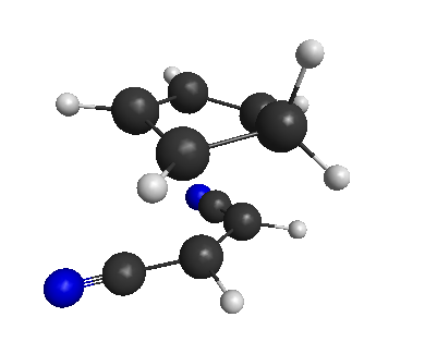
Optimized TS for the reaction
IRC calculation
The IRC calculation is done to make sure that the TS that we optimized actually leads to the reactant and product that we expect (from our chemical intuition). The IRC calculation from the optimized TS above was done in Part 5.
Here is the whole reaction path, from reactant to TS to product:
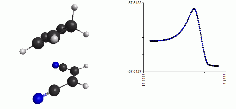
Full reaction coordinate with energy plot for the Diels-Alder reaction
As you can see, the mechanism is a concerted formation of two bonds, in one step. Here, the free energy of activation is just the difference between the free energy of the TS and the free energy of the reactant. (Note that the energy plot on the right is just the QM energy, it’s not the Gibbs free energy)
Reactant and Product optimization
We have the optimized TS, and we also have the IRC. All that is left to do is to perform the geometry optimization for the reactant and product state. Even though the IRC tries to reach the end of the reaction path on either side of the TS, it’s always necessary to run an optimization from the end points of the IRC, just to make sure that we have got the energy minima.
Optimization was covered in Part 1 and Part 2, so I will not go into detail here. Make GAMESS input files from the last points of both the forward and reverse IRC. Optimize them with PM6/SMD(dioxane) and OPTTOL=0.00005. Don’t forget to also request hessian calculation for the optimized structures with HSSEND=.t. in $STATPT. We will need the hessian calculation for the next step.
Thermochemistry at stationary points
The energy calculated by GAMESS is the sum of the electronic energy and the nuclear replusion energy (including the solvation free energy). However, Gibbs free energy contains terms of enthalpy and entropy. To estimate them, the energy contribution from the vibrational modes, and the rotational and translational motions has to be calculated. This is because, the optimization and IRC all assume that the temperature is 0 K, i.e. the atoms have zero kinetic energy. But at room temperature (298 K) the molecule has sufficient kinetic energy to rotate, move, or vibrate. Some approximations like ideal gas, harmonic approximation are used to calculate their contributions to the Gibbs free energy.
The exact mathematical details are not important here, but the bottom line is that the program automatically calculates all of this when the hessian is requested. This is why we added the HSSEND=.t. for all the optimizations.
Open the output files for the optimization with notepad, and scroll to the bottom. There should be something like this:

There are values for enthalpy(H), Gibbs free energy(G), entropy(S) etc. printed in two different units (kJ/mol and kcal/mol). We are interested in the Gibbs free energy, so we will only take that value in kcal/mol (63.881, indicated with red box). Note that this value is only a correction term, i.e. to obtain the actual Gibbs free energy, this term has to be added to the QM energy.
Free energy of activation
You can find the QM energy in the optimization log files. The easiest way is to open the files with wxMacMolPlt, and go to the final, optimized geometry. Then read the E value off the lower left corner. This gives the total QM energy for the system. (Also you can go to Molecule>Set Frame energy to get the energy with more significant figures). You can, of course, find the energy in the log file with notepad as well, but you have to read through some text to get to that.
Finally, add the QM energy to the Gibbs free energy correction term for each of reactant, TS and product. Be careful, because the QM energy is given in the units of Hartree (or a.u.) and that has to be converted to kcal/mol (1 Hartree = 627.5 kcal/mol) before adding.
For example, for the TS I got, QM energy=-57.57062347 Hartree=-36125.56623 kcal/mol and Gibbs free energy correction=59.579 kcal/mol. So that gives me final Gibbs free energy for TS=-36065.98723 kcal/mol.
Note that this value of the Gibbs free energy for one point does not really have any physical significance. Only the differences are relevant.
After doing the same calculation for the reactant, and product we get:
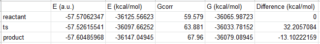
The difference between TS and reactant is the ΔG‡. The ΔG‡ calculated from experiment for this reaction is 21.2 kcal/mol. There is ~10 kcal/mol error in the value we calculated. This is expected because we used a semi-empirical method (PM6) in our calculation. These methods are usually parameterized to produce correct geometry, heats of formation etc. Predicting activation free energies is not their strength. Considering that, the 10 kcal/mol error is quite okay.
Can we improve the results?
Wait! we are not done. Let’s see if we can improve the calculated ΔG‡ value without recalculating everything. Since redoing the optimization and IRC using a more accurate method would take a lot of time, we can use the geometries that are optimized at PM6 level, and then calculate just the QM energies at a higher level. (Assuming that the geometries from PM6 are more or less accurate.)
This is done regularly in research, because usually the geometries are often already accurate at a lower level of theory, whereas accurate energies require higher level theories. In papers these type of calculations would be written as single point method//geometry and IRC method. For the calculation that we are about to do, it would be: M06–2X/pcseg-1//PM6 (pcseg-1 is a relatively recent basis set which has been optimized for DFT calculations, so it should give good results with M06–2X density functional).
Open the output files for geometry optimizations (for TS, reactant, and product) with MacMolPlt and write input files. Use RUNTYP=ENERGY to request a single point energy calculation. Also, put GBASIS=PCseg-1 in $BASIS and DFTTYP=M06–2X and ISPHER=1 in $CONTRL to set the method. Don’t forget to solvate the system in dioxane with SMD.
Since these are single point energy calculations with solvation model, GAMESS will perform two calculations, one in vacuum and one in solvent. MaxMolPlt will not give you the correct energy; you will have to open the log file and read it. At the very end of the log there should be a ‘total free energy in solvent’. This is the total QM energy (even though it reads free energy, it’s not the complete free energy).
Then we can replace the QM energies (E) with the values from the new calculation:
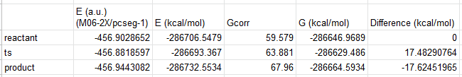
The activation energy is now 17.5 kcal/mol, so the error is ~4 kcal/mol. There is an immediate improvement.
Note that the G correction value comes from the vibrational analysis which is only valid at the same level of theory that we used to optimize the structures. So those values cannot be changed without reoptimizing.
Also keep in mind that semi-empirical methods are not used that much nowadays because of the upredictability of their errors, I used it here just to show you the way of doing the calculations.
Limitations
This scheme of calculations only gives valid results when there are no other factors that can contribute to the Gibbs free energies. So you have to be very careful. For example, if your reactant has a long chain, then it adds a chain entropy factor to the free energy (due to the large number of conformers). So if in the transition state, that chain is cut short/forms a ring then that chain entropy is lost, and GAMESS cannot automatically correct for that.
The bottom line is that the output from any QM program is correct, only as long as you have considered everything carefully.
wxMacMolPlt: https://brettbode.github.io/wxmacmolplt/
GAMESS: https://www.msg.chem.iastate.edu/gamess/